|
Linear System
Learner (LSLNR) |
The interactive root locus tool LSLNR plots the root locus
in one window and the closed loop step response in another window.
The GUI-window for the root locus allows students to change the
gain and also to move the compensator poles and zeros by clicking
on them and dragging them to new locations. The root locus and
the closed loop step response update automatically while the pole/zero
is being moved. This enables students to gain insight on how compensator
pole/zero locations affect the closed loop step response. It also
automates much of the iteration needed to fine-tune an initial
design that is based on dominant pole approximations.
|
Installation Instructions: |
This GUI has been tested with MATLAB ver. 5.2; it may not work
with later releases. The following are files that include both
root locus design and Bode plot design.
1) Create the subdirectory "LSLNR" in your MATLAB
toolbox directory and download the following files to this directory:
As an alternative, you can download the zipped files lslnr.zip
and use Winzip to unzip them.
2) Run Matlab and add the LSLNR directory to your path. This
will allow you to run the program without changing to the directory
each time.
3) That's it! Now that the files and path are installed and
established, follow the instructions on how to use the program.
|
Instructions for using
LSLNR: |
Brief Description:
At the Matlab prompt, type "cscra". This will bring
up the main window, "Linear System Command Center."
From this window, you can enter the poles and zeros of the plant
and compensator. This can be done in root or polynomial form.
(Note, if the window appears off of the screen, you may have
resize your display to 1024 x 768 or larger.)
The "Bode Design" button will generate an open loop
Bode magnitude and phase plot. You can add, delete or move compensator
poles/zeros.
The "Root Locus" button will plot the root locus
and allow you to modify the compensator by adding, deleting,
or moving the poles or zeros. From this window you can also modify
the gain. The pull-down menu labeled "Statistics" allows
you to view the corresponding closed loop pole positions along
with the damping ratio and natural frequency.
The closed loop step response is automatically generated.
Going to the "Performance" menu will allow you to display
the 2% settling time and other characteristics.
Detailed Description:
- I. Linear System Command Center Window
The linear system command center window allows the user to
enter roots or coefficients for the plant and compensator. The
user can specify which format to use by simply selecting the
appropriate radio button.
· Action Buttons
- Root Locus: This button generates a root locus
plot of the entire system.
- Bode Plot: This button generates a Bode magnitude
and phase plot.
- "+" and "-‘: These buttons
change the size of the plant and compensator displays.
· Radio Buttons
- Enter Poles and Zeros
Selecting this option allows the user to specify the plant
or compensator based on their poles or zeros.
- Enter Coefficients (default for both plant and
compensator)
Selecting this option will allow the user to enter the plant
and compensator in terms of the polynomial coefficients.
Note: Selecting either of the above radio buttons will
reset the edit fields to blank.
- Polynomial Form (default for plant):
Selecting this radio button will display the plant or compensator
in the form of a polynomial.
- Factored Form (default for compensator):
Selecting this option will display the plant or compensator
in terms of the factors of the numerator or denominator.
· Edit Fields
There are four edit fields in the form of two pairs. Each
pair represents the numerator and denominator of the compensator
and plant respectively. The fields are in tab order to allow
the user to quickly tab through the system entering process.
· Static Text
There are two static text field areas: one for displaying
the plant and another for displaying the compensator. By using
the "+" and "-" buttons, the systems display
can be adjusted to an appropriate size. This is especially useful
if the system has a large amount of complex roots and cannot
fit in the display area.
II. Root Locus Window
· Action Buttons
- Mouse: This button allows the user to set
the gain by clicking the mouse anywhere on the root-locus. Just
as in the manual case, once the gain is set, any window that
was open at the time is updated. The step response is always
re-plotted with the new gain. A new plot of the root locus is
generated with markers indicating the current position of the
roots.
- Add: Clicking this button will turn the mouse
pointer into a cross hair so that the user can specify where
on the root locus to place the new root(s). Based on the radio
button setting, real or complex roots will be added. If adding
complex roots, the conjugate root is automatically added. Only
one root needs to be specified. The addition of roots will only
affect the compensator and the compensator fields will be updated
with the new changes. All figures are updated with the change.
- Remove: Clicking this button will turn the
mouse pointer into a cross hair so that the user can specify
which root(s) on the graph is to be deleted. Only compensator
roots can be deleted- so once this button is clicked, the compensator
poles and zeros are bolded in black. Once the deletion is made,
the pointer changes back to an arrow and the compensator fields
are updated with the new changes. If complex roots are to be
deleted, once one root is specified, its conjugate is deleted
automatically. All figures are updated with the change.
- Move: Clicking this button will turn the cursor
into a fluer so that the user can specify which root on the graph
to move. This command only applies to compensator roots- so when
using this option, the compensator poles are bolded in black.
If complex poles are to be moved, once one root is specified,
its conjugate is automatically moved. The real axis can be crossed
while moving either complex pole. All figures are updated with
the change.
· Edit Fields
- There is one edit field that allows the user to enter the
gain manually. Once the user enters the new gain and hits the
return key, the same events result as if the mouse button was
used. This feature allows the user to specify explicit value
where as using the mouse allows you to specify a gain based on
indicating a current root position.
· Menu Options
- Statistics: This menu option allows the user
to view the current roots with respective z
and w n. If the root is
real, the z and w
n fields are filled with dashes.
-
III. Step Response Window
The step response window displays the step response and has
a menu option to display specific performance characteristics
(the menu option is appropriately named "Performance").
These characteristics are: Max % Overshoot, Peak Value,
Final Value, Rise-Time, 2% Settling Time,
and 5% Settling Time. As each one is selected, the menu
item is marked with a checkmark and the step response is marked
with a stem plot indicating the characteristic. For every subsequent
step response plot, the characteristics chosen will remain selected
until the user deselects them by going back to the "Performance"
menu and clicking on that item.
- IV. Bode Plot Window
The Bode plot window shows the magnitude and phase frequency
response, this is similar to the results obtained from the bode
command except for a few significant differences. The gain and
phase margins are indicated in the window along with the gain
a phase crossover points. The crossover points also indicate
the actual frequency of the crossover. The action buttons (add,
move, etc.) work the same as those in the root locus window.
The only major difference here is in the gain button. The gain
entered into the gain field is the DC gain (for a Type 0 system)
in decibels. In other words, put the transfer function into the
standard form used for Bode design. The open loop gain should
be entered into the field. For example, if the plant and compensator
are defined as
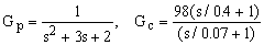
then enter 20log(49) into the gain field or enter 98 as part
of the compensator. If the latter procedure is followed, then
20log(49) will automatically be displayed in the gain field.