Additions or changes to this page might not show up on your computer if you have an older version in your internet cache. You may wish to click on the Refresh button in your browser to be certain that you see any changes.
The text for the class is "Introduction Electroacoustics & Audio Amplifier Design" by W. Marshall Leach, Jr., ISBN 0-7575-0375-6.
Before coming into my office, please turn your cell phone off.
Making the Grade by Physics Professor Kurt Weisenfeld. You can read a student's response here.
Chapters 1 - 12 Formula Sheet Use of this is allowed on quizzes. No additional material may be written on it. Additions or corrections may be made before quizzes.
Electroacoustics Glossary of Symbols. You may use a copy of this on the quizzes. No additional material may be written on it.
The Perception of Pitch. The pitch of a sound wave is closely related to its frequency or periodicity - but the exact nature of that relation remains a mystery. A very interesting article from the 1974 issue of American Scientist published by Sigma Xi.
A paper that describes the design of Zobel matching networks can be read here. You can read see the Mathcad sheet which was used to produce the plots in Figures 7 and 8 in the paper here.
The following links are to the numerical tables from which the vented-box design charts in the book were plotted: QL = 03, QL = 05, QL = 07, QL = 10, QL = 20, QL = infinity
SPICE Netlists: Infinite-Baffle, Closed-Box, Vented-Box
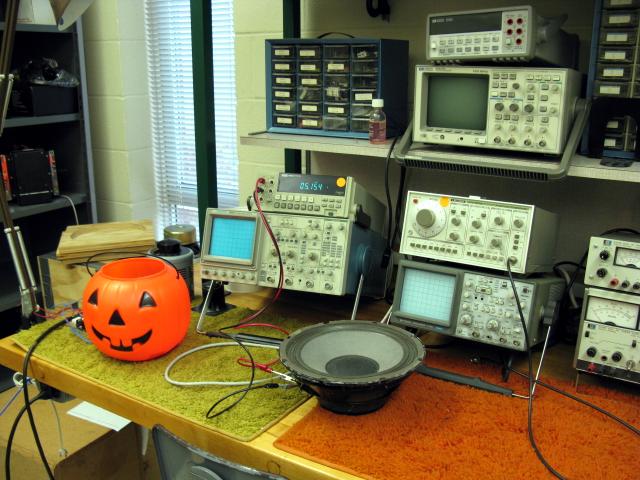
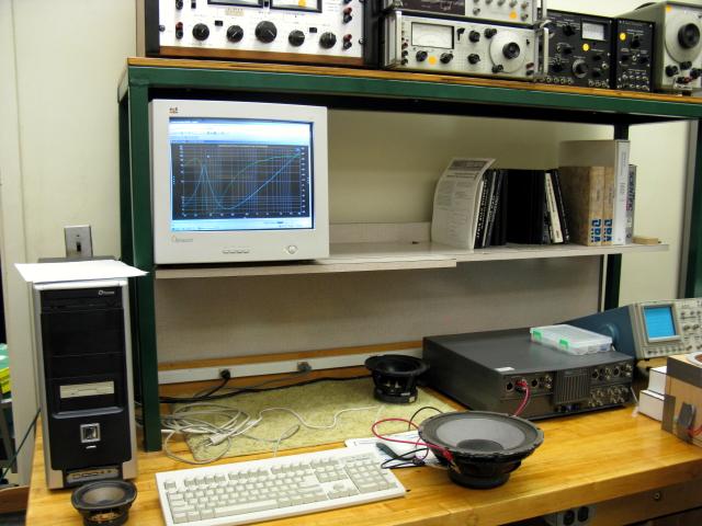
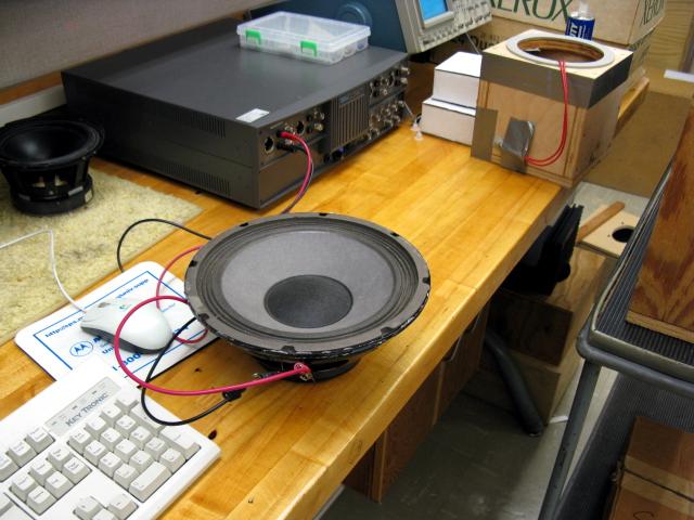
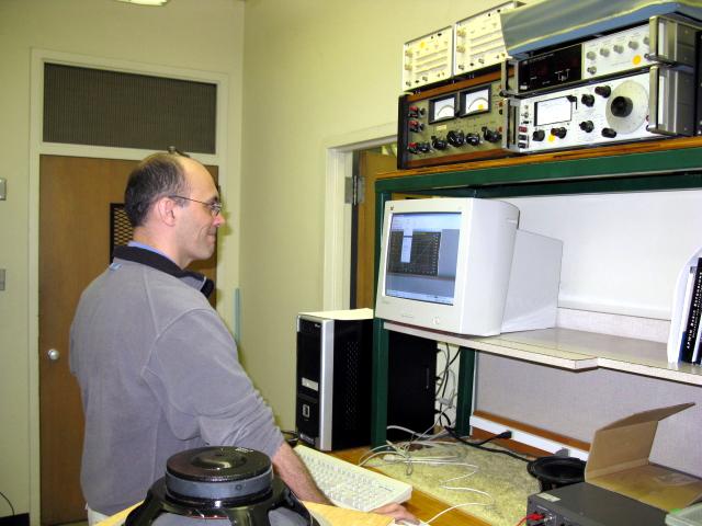
The following pictures show the laboratory setup for measuring the voice-coil impedance of loudspeakers. The basic instrument is the computer controlled Audio Precision Analyzer II.
Picture 01 - Measuring the voice-coil resistance with the ohmmeter.
Picture 02 - Loudspeaker driver connected to the Audio Precision Analyzer II.
Picture 03 - Closeup view of the speaker and analyzer.
Picture 04 - Dr. Allen Robinson making the measurements.
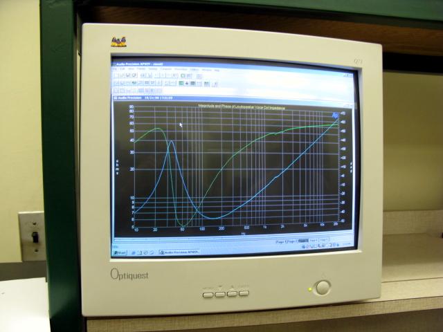
Picture 05 - Screenshot showing the measured magnitude and phase of the impedance.
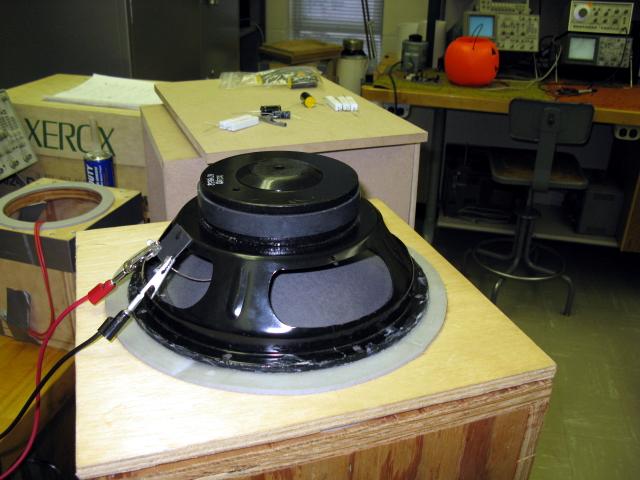
Picture 06 - The loudspeaker mounted on the compliance test box.
The SPICE examples in the 4th edition of the text used LTSpice for the analysis. This version of SPICE is distributed by Linear Technology and has become the defacto standard for the "do it yourself" electronics and audio communities. Unlike other free versions, there are no limits on the number of devices in a circuit. Here are the links:
Linear Technology Software Page
LTSpice Tutorial
LTSpice Guide
These are the LTSpice files that are in the 4th edition of the text. The crossover network example contains both a woofer and a midrange driven from a single power amplifier with crossover networks. There is an auxiliary RLC circuit that connects to the midrange voice coil for impedance correction.
Infinite Baffle File from Chapter 6.
Closed-Box File from Chapter 7.
Vented-Box File from Chapter 8.
Crossover Example File from Chapter 10.
This paper explains the equations in the mathcad sheet that are used to determine the inductor parameters.
The design of Zobel networks to cancel the high-frequency rise in voice coil impedance due to the inductnce is described in this paper.
Errata and Updates for Course Text - Student assistance in finding errors will be appreciated.
Read this copy of a paper on modeling the voice-coil inductance losses. This paper explains the equations on the mathcad sheet that are used to determine the inductor parameters.
Parameter Calculation Sheet for calculating the small-signal parameters of the driver. You must read Section 12.7 in the text to understand this sheet. The only parts that pertain to the design project are the parts where you calculate fS, QMS, QES, QTS, and VAS.
Here is a free version of SPICE that you might like better than PSpice. The evaluation version lets you have 20 active devices (PSpice only allows 10) and 50 nodes in a circuit. The program makes better use of the graphics features of Windows. For example, you can copy plots to the clipboard as metafiles, whereas PSpice only lets you make bitmaps of plots (if you can figure out how to do it). With the graphics post processor, you can scale the plots with the mouse, control the labeling and gridlines, change the axis labels, etc., things that cannot be done with PSpice. You can download the free evaluation version of AIM Spice here.

This page is not a publication of the Georgia Institute of Technology and the Georgia Institute of Technology has not edited or examined the content. The author of this page is solely responsible for the content.